-
Exercise Title: Raster Scales and Vector Resolution
-
Abstract: A table published by SCANEX.RU is offered as an example of how satellite raster images are referred to "scales" when published. Scales are widely cited in environmental literature and management documents, and this table allows users to make rough approximations of the pixel sizes of remotely-sensed images that meet these requirements. Then a method is described for roughly estimating the "resolutions" of vector objects, based on the numbers of data points needed to draw mapped features. This method is appropriate for natural features only, but might yield too-large resolution values for political or cultural features, due to long, straight lines with few points.
-
Preliminary Reading (in OceanTeacher, unless otherwise indicated):
-
Scale (Map) - Wikipedia article
-
Image Resolution and Map Scales - SCANEX.RU website paper, with useful tables relating imaging systems to reporting scales for topographic maps and thematic maps. Range of scales from 1:10,000 to 1:1,000,000, for pixel sizes ranging from less than a meter to hundreds of meters.
-
Remote Sensing Resources - American Museum article defining satellite image resolution
-
Required Software:
-
Other Resources:
-
Author: Murray Brown
-
Version: 3-10-2015
This table is probably a good general reference, as long as it is not taken to be rigorous, but just suggestive. Read the original paper to see more than this condensed view.
|
Pixel Size(m) |
"Scale" |
||||||
| 10K-25K | 25K-50K | 50K-100K | 100K-200K | 200K-500K | 500K-1M | >1M | |
| 250-1000 | |||||||
| 140 | |||||||
| 35-45 | |||||||
| 30 | |||||||
| 25-30 | |||||||
| 23.5 | |||||||
| 23.5 | |||||||
| 20 | |||||||
| 15-30 | |||||||
| 15 | |||||||
| 10 | |||||||
| 5.8 | |||||||
| 5 | |||||||
| 5 | |||||||
| 2-2.8 | |||||||
| 0.8 | |||||||
"For pixel based products, you can determine the appropriate resolution necessary for your applications based upon the smallest feature you want to resolve (i.e. Minimum Mapping Unit). The pixel size must be half the smallest dimension of the feature in question. For instance if you want to find a car (which would be ~10 feet x 6 feet), then the smallest dimension of that car is 6 feet, so your pixel size must be no larger 3 x 3 feet to reliably identify and map cars." [NCSC Digital Coast]
NOTE: ENC = Electronic Navigation Chart
NOTE2: NM = nautical mile ~ 1.8 km
| Serie selezionabile | Scala di compilazione standard delle ENCs | Chart Type Name (from Chilean Hydrographic Charts Catalog) |
| 200 NM | 1:3,000,000 | General Overview |
| 96 NM | 1:1,500,000 | |
| 48 NM | 1:700,000 | Ocean |
| 24 NM | 1:350,000 | |
| 12 NM | 1:180,000 | |
| 6 NM | 1:90,000 | Coast |
| 3 NM | 1:45,000 | |
| 1.5 NM | 1:22,000 | Approach |
| 0.75 NM | 1:12,000 | Port |
| 0.5 NM | 1:8,000 | |
| 0.25 NM | 1:4,000 | |
| (>1:4000) | Pier |
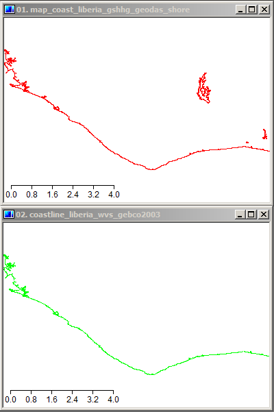
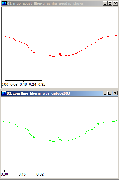
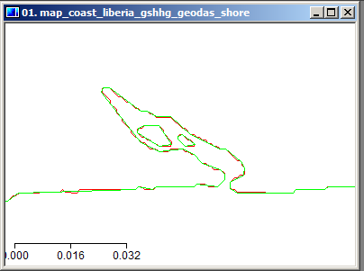
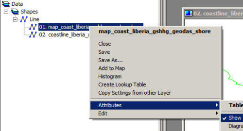
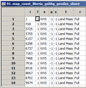
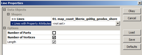
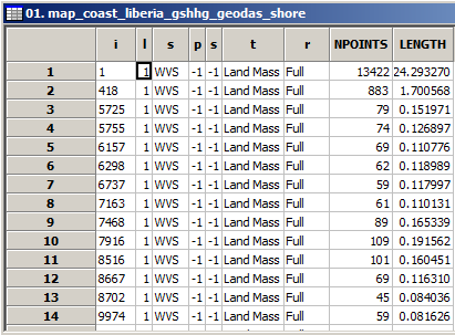
- NPOINTS - The number of points in each section of the line shape
- LENGTH - The length of each section
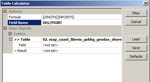
- Enter a new field name such as DEG/POINT to indicate a new measure of the ratio of length (DEG) to data (POINTS)
- For TABLE, select the GSHHG shape
Then click OK to add this new field to the data table.
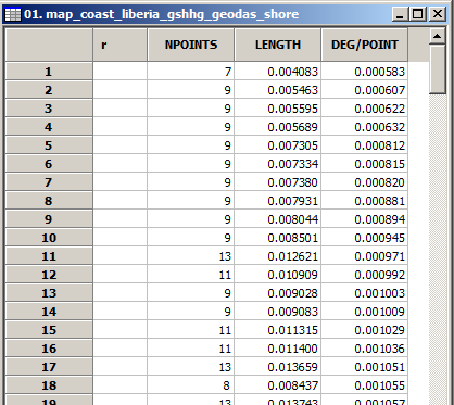
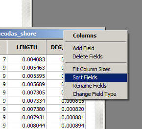
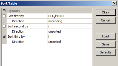
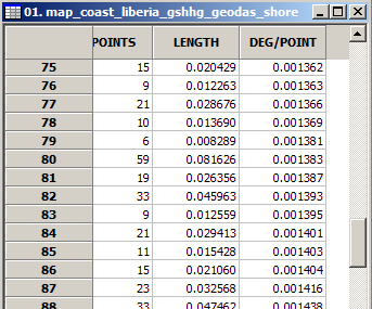
- The DEG/POINT values at the top of the table begin at roughly 0.0006
- The values near the middle (second image) include the MEDIAN at location 80, with a value of roughly 0.0014 DEG/POINT.
- The values at the bottom of the table increase sharply to a high value of 0.0054 DEG/POINT.
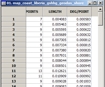 |
 |
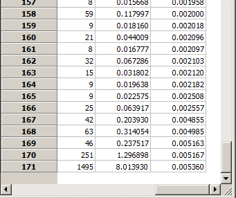 |
The full range of resolutions goes from about 41 m to 540 m, but the minima and maxima "tails" in this distribution are very limited, so a simple visual evaluation of the median is quite justified.
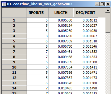
- The values at the top of the table sharply increase from the lowest value of 0.0010
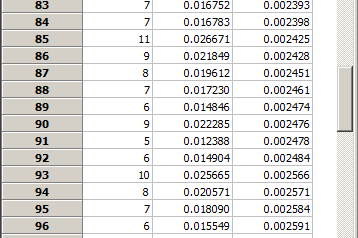
- The values near the middle (second image) include the MEDIAN at location 90, with a value of 0.0025 degrees.
- The values at the bottom of the table increase sharply to a high value of 0.0057
 |
 |
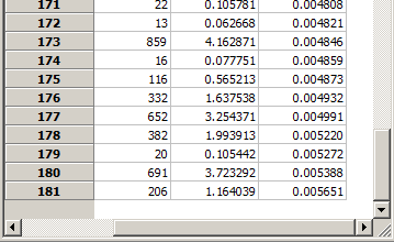 |
The full range of resolutions goes from about 50 m to 570 m, but the minima and maxima "tails" in this distribution are very limited, so a simple visual evaluation of the median is quite justified.